Statistics#
Test every assay of the analysis table, with one method chosen up front, effect sizes with 95% intervals, and an FDR (Benjamini-Hochberg) over all tested assays.
Both test functions take the table from to_wide (or any table
with proteins=[...] given) and return a StatsResult: it prints as a report, and holds the
tables .table (one row per assay, sorted by p), .pairwise (three or more groups) and
.not_tested (assays left out, with the reason; they stay out of the FDR).
compare_groups#
Compare NPX between groups, assay by assay.
compare_groups(table, group, *, test="welch", reference=None, ordered=False, order=None,
               proteins=None, below_lod=None, alpha=0.05, level=0.95,
               verbose=True) -> StatsResult
| Argument | Type | Default | Meaning |
|---|---|---|---|
table |
DataFrame | — | the analysis table |
group |
str | — | the column with the groups, e.g. "diabetes"; samples without a group are left out and counted |
test |
str | "welch" |
"welch": Welch's t-test (two groups) or Welch's ANOVA (three or more); "mann-whitney": Mann-Whitney U or Kruskal-Wallis |
reference |
required | the group the others are compared with, e.g. "control". Every difference is "other group minus reference", so it sets the sign of every result. With three or more groups, pairs without the reference subtract the earlier group (in order, else alphabetical) |
|
ordered |
bool | False |
the groups have a natural order: one trend test (a line with robust HC3 errors for Welch; Jonckheere-Terpstra for Mann-Whitney) |
order |
list | None |
the groups in their order, for ordered=True, e.g. ["normal", "prediabetes", "diabetes"] |
proteins |
list | None |
the assay columns; default from to_wide |
below_lod |
DataFrame | None |
to_wide(..., values="below_lod"): adds the share below the LOD per group |
alpha |
float | 0.05 |
the FDR level used in the report |
level |
float | 0.95 |
the level of the intervals |
Output per assay (.table): n_ and mean_ per group (median_ for Mann-Whitney);
two groups: difference (in NPX, the log2 fold change; the Hodges-Lehmann shift for
Mann-Whitney) with ci_low / ci_high; three or more groups: statistic; an ordered trend:
slope with its interval; then p and fdr. With three or more groups, .pairwise compares
every pair, Holm-adjusted within each assay: read it for the assays whose FDR is below alpha.
Why one test for every assay. Choosing a test per assay after a normality test makes the choice follow the sample size more than the data, and mixes different tests in one FDR. Welch's tests allow each group its own spread, which keeps the error rate right when groups differ in size and spread.
Errors. ValueError for fewer than two groups, a group with fewer than 2 samples,
no reference, an unknown test, or ordered=True without an order. KeyError when group is missing from
the table.
correlate#
Correlate NPX with a continuous variable, assay by assay.
correlate(table, variable, *, method="spearman", proteins=None, alpha=0.05, level=0.95,
          verbose=True) -> StatsResult
| Argument | Type | Default | Meaning |
|---|---|---|---|
variable |
str | — | the column with the continuous variable, e.g. "age"; samples without a value are left out and counted |
method |
str | "spearman" |
"spearman": any rising or falling relation, robust to extreme values; "pearson": a straight-line relation |
Output per assay (.table): n, r with ci_low / ci_high (Fisher's z; for Spearman
with the Bonett-Wright standard error), p, fdr.
plot_volcano#
Every assay of a result at once: the effect (x) against how certain it is (y, -log10 p).
For two groups x is the difference (log2 fold change), for a trend the slope, for a
correlation r. Assays with an FDR below alpha are coloured, and the strongest labels of them
are named; the dotted line marks the FDR cutoff.
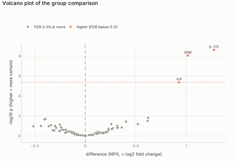
plot_volcano(compare_groups(table, "group", reference="control")) on the synthetic data: IL-17C, OSM and IL6 are higher in cases.
fdr_bh, holm#
Adjust a list of p-values. Missing p-values stay missing and do not count in the family.
The lessons: Compare groups, Correlate.