Start

Start in 5 minutes

The four preprocessing steps on synthetic NPX data that comes with signatomics, so you get exactly the output shown here.

1. Install

pip install "signatomics[olink] @ git+https://github.com/ElenaStamatelou/signatomics"

Needs Python 3.10 or newer. signatomics installs from GitHub until it is on the Python package index; [olink] adds what the Olink part needs (reading .xlsx and .parquet files, charts).

2. Data import

import signatomics.olink as so

data = so.read_npx(so.example_file())      # your own file: so.read_npx("my_npx_file.csv")

so.example_file() gives the path to a synthetic NPX file that comes with signatomics: one Target 96 plate with 40 samples, 8 controls and 92 assays. Synthetic means the values are generated to look like real Olink data, without any person or study behind them.

On the synthetic example file

Reading report
  file: example_plate1.csv
  file type: .csv
  layout: long format (one row per sample and assay)
  control samples: 8 (marked in SampleType); apply_qc removes them
  result: 4416 rows = (40 samples + 8 controls) x 92 assays

Whatever the NPX file looks like (long or wide format; .csv, .txt, .xlsx or .parquet), every function works on the same table in long format, with Olink's column names. In blue: one measurement. In the wide file its details sit in different places; in long format they share one row. All other Olink columns (OlinkID, UniProt, Panel, ...) are kept. Values are synthetic.

3. Quality control

so.qc_report(data)                # look: your data stays as it is
so.plot_npx_strip(data)           # every value per assay, with the LOD
clean = so.apply_qc(data)         # act: removes controls and FAIL samples

On the synthetic example file

Quality report
  controls (left out of the checks below; apply_qc removes them): 8 control samples (3 NEGATIVE_CONTROL, 3 PLATE_CONTROL, 2 SAMPLE_CONTROL)
  data: 40 samples, 92 assays, 1 plate
  QC status: 38 PASS, 1 WARN, 1 FAIL
  assays below the LOD in more than 75% of the samples: 11 of 92 (a sign of data quality; they stay in)
  outliers: 1 of 40 samples (P07); see plot_sample_qc

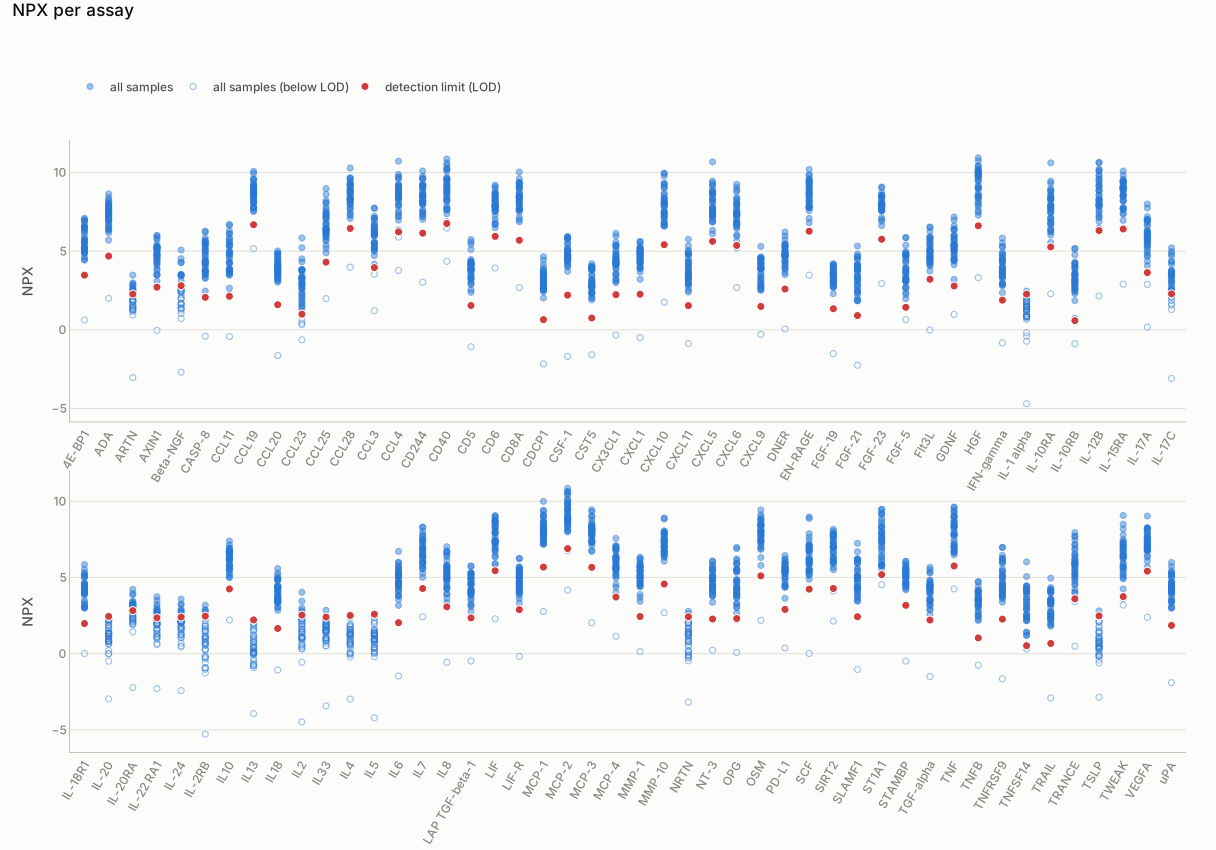
so.plot_npx_strip(data). Each dot is one sample's NPX value for one assay; the red dot is the assay's detection limit (LOD), and hollow dots lie below it. Hover a dot for its value.

4. Bridging optional: for samples on several plates

The example has a second plate; 12 samples are on both.

import pandas as pd

both = pd.concat([so.read_npx(so.example_file(1)), so.read_npx(so.example_file(2))],
                 ignore_index=True)
clean = so.apply_qc(both)
combined = so.bridge_plates(clean)     # plate 2 on the scale of plate 1

On the synthetic example files

Bridging report
  reference (kept as it is): Plate 1
  Plate 2: 92 assays adjusted by their adjustment factor (median -0.51 NPX, from -1.67 to +1.05), each from 12 bridge samples
  ...

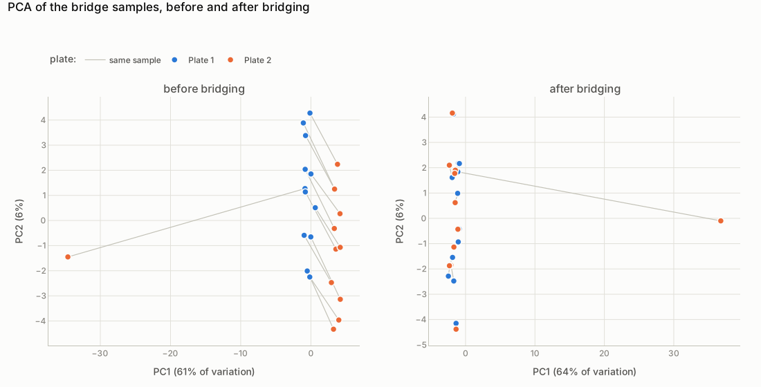
so.plot_bridge_pca(clean, combined). Each line joins one bridge sample's two measurements: after bridging they lie together and the plates overlap. The point far from the rest is P33, the broken tube.

5. Sample metadata

data = so.add_sample_info(combined, so.example_samples(), on="sample_id")

On the synthetic example files

Matching report
  matched on: SampleID (NPX data) = sample_id (your sample metadata)
  matched: 59 of 59 sample IDs in the NPX data
  missing from the NPX data: P20

Your sample metadata (demographics, clinical data, ...) now sits next to the NPX values. P20 is missing because quality control removed it (QC status FAIL).

All of it in one call

data = so.prepare([so.example_file(1), so.example_file(2)], so.example_samples(), on="sample_id")

prepare runs the four steps with their default choices and prints one short report, with a list of what to look at yourself (such as the outlier P07). See In one call.

Next

• Learn: each step on its own, and what its output means.
• Functions: every function with all its options.
• Examples: the same steps on real Olink studies.